Analyze Data With LangChain AI Agent

このコンテンツはまだ日本語訳がありません。

This package provides the DaytonaDataAnalysisTool - LangChain tool integration that enables agents to perform secure Python data analysis in a sandboxed environment. It supports multi-step workflows, file uploads/downloads, and custom result handling, making it ideal for automating data analysis tasks with LangChain agents.

This page demonstrates the use of this tool with a basic example analyzing a vehicle valuations dataset. Our goal is to analyze how vehicle prices vary by manufacturing year and create a line chart showing average price per year.

1. Workflow Overview

You upload your dataset and provide a natural language prompt describing the analysis you want. The agent reasons about your request, determines how to use the DaytonaDataAnalysisTool to perform the task on your dataset, and executes the analysis securely in a Daytona sandbox.

You provide the data and describe what insights you need - the agent handles the rest.

2. Project Setup

2.1 Install Dependencies

Install the required packages for this example:

Python

pip install -U langchain langchain-anthropic langchain-daytona-data-analysis python-dotenv

The packages include:

langchain: LangChain framework for building AI agents
langchain-anthropic: Integration package connecting Claude (Anthropic) APIs and LangChain
langchain-daytona-data-analysis: Provides the DaytonaDataAnalysisTool for LangChain agents
python-dotenv: Used for loading environment variables from .env file

2.2 Configure Environment

Get your API keys and configure your environment:

Daytona API key: Get it from Daytona Dashboard
Anthropic API key: Get it from Anthropic Console

Create a .env file in your project:

DAYTONA_API_KEY=dtn_***
ANTHROPIC_API_KEY=sk-ant-***

3. Download Dataset

We’ll be using a publicly available dataset of vehicle valuation. You can download it directly from:

https://download.daytona.io/dataset.csv

Download the file and save it as vehicle-dataset.csv in your project directory.

4. Initialize the Language Model

Models are the reasoning engine of LangChain agents - they drive decision-making, determine which tools to call, and interpret results.

In this example, we’ll use Anthropic’s Claude model, which excels at code generation and analytical tasks.

Configure the Claude model with the following parameters:

Python

from langchain_anthropic import ChatAnthropic

model = ChatAnthropic(
    model_name="claude-sonnet-4-5-20250929",
    temperature=0,
    max_tokens_to_sample=1024,
    timeout=None,
    max_retries=2,
    stop=None
)

Parameters explained:

model_name: Specifies the Claude model to use
temperature: Tunes the degree of randomness in generation
max_tokens_to_sample: Number of tokens to predict per generation
max_retries: Number of retries allowed for Anthropic API requests

5. Define the Result Handler

When the agent executes Python code in the sandbox, it generates artifacts like charts and output logs. We can define a handler function to process these results.

This function will extract chart data from the execution artifacts and save them as PNG files:

Python

import base64
from daytona import ExecutionArtifacts

def process_data_analysis_result(result: ExecutionArtifacts):
    # Print the standard output from code execution
    print("Result stdout", result.stdout)

    result_idx = 0
    for chart in result.charts:
        if chart.png:
            # Charts are returned in base64 format
            # Decode and save them as PNG files
            with open(f'chart-{result_idx}.png', 'wb') as f:
                f.write(base64.b64decode(chart.png))
            print(f'Chart saved to chart-{result_idx}.png')
            result_idx += 1

This handler processes execution artifacts by:

Logging stdout output from the executed code
Extracting chart data from the artifacts
Decoding base64-encoded PNG charts
Saving them to local files

6. Configure the Data Analysis Tool

Now we’ll initialize the DaytonaDataAnalysisTool and upload our dataset.

Python

from langchain_daytona_data_analysis import DaytonaDataAnalysisTool

# Initialize the tool with our result handler
DataAnalysisTool = DaytonaDataAnalysisTool(
    on_result=process_data_analysis_result
)

try:
  # Upload the dataset with metadata describing its structure
  with open("./vehicle-dataset.csv", "rb") as f:
      DataAnalysisTool.upload_file(
          f,
          description=(
              "This is a CSV file containing vehicle valuations. "
              "Relevant columns:\n"
              "- 'year': integer, the manufacturing year of the vehicle\n"
              "- 'price_in_euro': float, the listed price of the vehicle in Euros\n"
              "Drop rows where 'year' or 'price_in_euro' is missing, non-numeric, or an outlier."
          )
      )

Key points:

The on_result parameter connects our custom result handler
The description provides context about the dataset structure to the agent
Column descriptions help the agent understand how to process the data
Data cleaning instructions ensure quality analysis

7. Create and Run the Agent

Finally, we’ll create the LangChain agent with our configured model and tool, then invoke it with our analysis request.

Python

from langchain.agents import create_agent

# Create the agent with the model and data analysis tool
agent = create_agent(model, tools=[DataAnalysisTool], debug=True)

    # Invoke the agent with our analysis request
    agent_response = agent.invoke({
        "messages": [{
            "role": "user",
            "content": "Analyze how vehicles price varies by manufacturing year. Create a line chart showing average price per year."
        }]
    })
finally:
    # Always close the tool to clean up sandbox resources
    DataAnalysisTool.close()

What happens here:

The agent receives your natural language request
It determines it needs to use the DaytonaDataAnalysisTool
Agent generates Python code to analyze the data
Code executes securely in the Daytona sandbox
Results are processed by our handler function
Charts are saved to your local directory
Sandbox resources are cleaned up in the finally block

8. Running Your Analysis

Now you can run the complete code to see the results.

Python

python data-analysis.py

Understanding the Agent’s Execution Flow

When you run the code, the agent works through your request step by step. Here’s what happens in the background:

Step 1: Agent receives and interprets the request

The agent acknowledges your analysis request:

AI Message: "I'll analyze how vehicle prices vary by manufacturing year and create a line chart showing the average price per year."

Step 2: Agent generates Python code

The agent generates Python code to explore the dataset first:

import pandas as pd
import matplotlib.pyplot as plt
import numpy as np

# Load the dataset
df = pd.read_csv('/home/daytona/vehicle-dataset.csv')

# Display basic info about the dataset
print("Dataset shape:", df.shape)
print("\nFirst few rows:")
print(df.head())
print("\nColumn names:")
print(df.columns.tolist())
print("\nData types:")
print(df.dtypes)

Step 3: Code executes in Daytona sandbox

The tool runs this code in a secure sandbox and returns the output:

Result stdout Dataset shape: (100000, 15)

First few rows:
   Unnamed: 0  ...                               offer_description
0       75721  ...  ST-Line Hybrid Adapt.LED+Head-Up-Display Klima
1       80184  ...             blue Trend,Viele Extras,Top-Zustand
2       19864  ...    35 e-tron S line/Matrix/Pano/ACC/SONOS/LM 21
3       76699  ...           2.0 Lifestyle Plus Automatik Navi FAP
4       92991  ...                    1.6 T 48V 2WD Spirit LED, WR

[5 rows x 15 columns]

Column names:
['Unnamed: 0', 'brand', 'model', 'color', 'registration_date', 'year',
 'price_in_euro', 'power_kw', 'power_ps', 'transmission_type', 'fuel_type',
 'fuel_consumption_l_100km', 'fuel_consumption_g_km', 'mileage_in_km',
 'offer_description']

Data types:
Unnamed: 0                    int64
brand                        object
model                        object
color                        object
registration_date            object
year                         object
price_in_euro                object
power_kw                     object
power_ps                     object
transmission_type            object
fuel_type                    object
fuel_consumption_l_100km     object
fuel_consumption_g_km        object
mileage_in_km               float64
offer_description            object
dtype: object

Step 4: Agent generates detailed analysis code

Based on the initial dataset information, the agent generates more specific code to examine the key columns:

import pandas as pd
import matplotlib.pyplot as plt
import numpy as np

# Load the dataset
df = pd.read_csv('/home/daytona/vehicle-dataset.csv')

print("Dataset shape:", df.shape)
print("\nColumn names:")
print(df.columns.tolist())

# Check for year and price_in_euro columns
print("\nChecking 'year' column:")
print(df['year'].describe())
print("\nMissing values in 'year':", df['year'].isna().sum())

print("\nChecking 'price_in_euro' column:")
print(df['price_in_euro'].describe())
print("\nMissing values in 'price_in_euro':", df['price_in_euro'].isna().sum())

Step 5: Execution results from sandbox

The code executes and returns column statistics:

Result stdout Dataset shape: (100000, 15)

Column names:
['Unnamed: 0', 'brand', 'model', 'color', 'registration_date', 'year',
 'price_in_euro', 'power_kw', 'power_ps', 'transmission_type', 'fuel_type',
 'fuel_consumption_l_100km', 'fuel_consumption_g_km', 'mileage_in_km',
 'offer_description']

Checking 'year' column:
count     100000
unique        49
top         2019
freq       12056
Name: year, dtype: object

Missing values in 'year': 0

Checking 'price_in_euro' column:
count     100000
unique     11652
top        19990
freq         665
Name: price_in_euro, dtype: object

Missing values in 'price_in_euro': 0

Step 6: Agent generates final analysis and visualization code

Now that the agent understands the data structure, it generates the complete analysis code with data cleaning, processing, and visualization:

import pandas as pd
import matplotlib.pyplot as plt
import numpy as np

# Load the dataset
df = pd.read_csv('/home/daytona/vehicle-dataset.csv')

print("Original dataset shape:", df.shape)

# Clean the data - remove rows with missing values in year or price_in_euro
df_clean = df.dropna(subset=['year', 'price_in_euro'])
print(f"After removing missing values: {df_clean.shape}")

# Convert to numeric and remove non-numeric values
df_clean['year'] = pd.to_numeric(df_clean['year'], errors='coerce')
df_clean['price_in_euro'] = pd.to_numeric(df_clean['price_in_euro'], errors='coerce')

# Remove rows where conversion failed
df_clean = df_clean.dropna(subset=['year', 'price_in_euro'])
print(f"After removing non-numeric values: {df_clean.shape}")

# Remove outliers using IQR method for both year and price
def remove_outliers(df, column):
    Q1 = df[column].quantile(0.25)
    Q3 = df[column].quantile(0.75)
    IQR = Q3 - Q1
    lower_bound = Q1 - 1.5 * IQR
    upper_bound = Q3 + 1.5 * IQR
    return df[(df[column] >= lower_bound) & (df[column] <= upper_bound)]

df_clean = remove_outliers(df_clean, 'year')
print(f"After removing year outliers: {df_clean.shape}")

df_clean = remove_outliers(df_clean, 'price_in_euro')
print(f"After removing price outliers: {df_clean.shape}")

print("\nCleaned data summary:")
print(df_clean[['year', 'price_in_euro']].describe())

# Calculate average price per year
avg_price_by_year = df_clean.groupby('year')['price_in_euro'].mean().sort_index()

print("\nAverage price by year:")
print(avg_price_by_year)

# Create line chart
plt.figure(figsize=(14, 7))
plt.plot(avg_price_by_year.index, avg_price_by_year.values, marker='o',
         linewidth=2, markersize=6, color='#2E86AB')
plt.xlabel('Manufacturing Year', fontsize=12, fontweight='bold')
plt.ylabel('Average Price (€)', fontsize=12, fontweight='bold')
plt.title('Average Vehicle Price by Manufacturing Year', fontsize=14,
          fontweight='bold', pad=20)
plt.grid(True, alpha=0.3, linestyle='--')
plt.xticks(rotation=45)

# Format y-axis to show currency
ax = plt.gca()
ax.yaxis.set_major_formatter(plt.FuncFormatter(lambda x, p: f'€{x:,.0f}'))

plt.tight_layout()
plt.show()

# Additional statistics
print(f"\nTotal number of vehicles analyzed: {len(df_clean)}")
print(f"Year range: {int(df_clean['year'].min())} - {int(df_clean['year'].max())}")
print(f"Price range: €{df_clean['price_in_euro'].min():.2f} - €{df_clean['price_in_euro'].max():.2f}")
print(f"Overall average price: €{df_clean['price_in_euro'].mean():.2f}")

This comprehensive code performs data cleaning, outlier removal, calculates averages by year, and creates a professional visualization.

Step 7: Final execution and chart generation

The code executes successfully in the sandbox, processes the data, and generates the visualization:

Result stdout Original dataset shape: (100000, 15)
After removing missing values: (100000, 15)
After removing non-numeric values: (99946, 15)
After removing year outliers: (96598, 15)
After removing price outliers: (90095, 15)

Cleaned data summary:
               year  price_in_euro
count  90095.000000   90095.000000
mean    2016.698563   22422.266707
std        4.457647   12964.727116
min     2005.000000     150.000000
25%     2014.000000   12980.000000
50%     2018.000000   19900.000000
75%     2020.000000   29500.000000
max     2023.000000   62090.000000

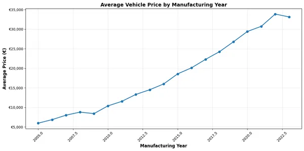
Average price by year:
year
2005.0     5968.124319
2006.0     6870.881523
2007.0     8015.234473
2008.0     8788.644495
2009.0     8406.198576
2010.0    10378.815972
2011.0    11540.640435
2012.0    13306.642261
2013.0    14512.707025
2014.0    15997.682899
2015.0    18563.864358
2016.0    20124.556294
2017.0    22268.083322
2018.0    24241.123673
2019.0    26757.469111
2020.0    29400.163494
2021.0    30720.168646
2022.0    33861.717552
2023.0    33119.840175
Name: price_in_euro, dtype: float64

Total number of vehicles analyzed: 90095
Year range: 2005 - 2023
Price range: €150.00 - €62090.00
Overall average price: €22422.27

Chart saved to chart-0.png

The agent successfully completed the analysis, showing that vehicle prices generally increased from 2005 (€5,968) to 2022 (€33,862), with a slight decrease in 2023. The result handler captured the generated chart and saved it as chart-0.png.

You should see the chart in your project directory that will look similar to this:

Vehicle valuation by manufacturing year chart

9. Complete Implementation

Here is the complete, ready-to-run example:

Python

import base64
from dotenv import load_dotenv
from langchain.agents import create_agent
from langchain_anthropic import ChatAnthropic
from daytona import ExecutionArtifacts
from langchain_daytona_data_analysis import DaytonaDataAnalysisTool

load_dotenv()

model = ChatAnthropic(
  model_name="claude-sonnet-4-5-20250929",
  temperature=0,
  max_tokens_to_sample=1024,
  timeout=None,
  max_retries=2,
  stop=None
)

def process_data_analysis_result(result: ExecutionArtifacts):
  # Print the standard output from code execution
  print("Result stdout", result.stdout)
  result_idx = 0
  for chart in result.charts:
      if chart.png:
          # Save the png to a file
          # The png is in base64 format.
          with open(f'chart-{result_idx}.png', 'wb') as f:
              f.write(base64.b64decode(chart.png))
          print(f'Chart saved to chart-{result_idx}.png')
          result_idx += 1

def main():
  DataAnalysisTool = DaytonaDataAnalysisTool(
      on_result=process_data_analysis_result
  )

  try:
      with open("./vehicle-dataset.csv", "rb") as f:
          DataAnalysisTool.upload_file(
              f,
              description=(
                  "This is a CSV file containing vehicle valuations. "
                  "Relevant columns:\n"
                  "- 'year': integer, the manufacturing year of the vehicle\n"
                  "- 'price_in_euro': float, the listed price of the vehicle in Euros\n"
                  "Drop rows where 'year' or 'price_in_euro' is missing, non-numeric, or an outlier."
              )
          )

      agent = create_agent(model, tools=[DataAnalysisTool], debug=True)

      agent_response = agent.invoke(
          {"messages": [{"role": "user", "content": "Analyze how vehicles price varies by manufacturing year. Create a line chart showing average price per year."}]}
      )
  finally:
      DataAnalysisTool.close()

if __name__ == "__main__":
  main()

Key advantages of this approach:

Secure execution: Code runs in isolated Daytona sandbox
Automatic artifact capture: Charts, tables, and outputs are automatically extracted
Natural language interface: Describe analysis tasks in plain English
Framework integration: Seamlessly works with LangChain’s agent ecosystem

10. API Reference

The following public methods are available on DaytonaDataAnalysisTool:

download_file

def download_file(remote_path: str) -> bytes

Downloads a file from the sandbox by its remote path.

Arguments:

remote_path - str: Path to the file in the sandbox.

Returns:

bytes - File contents.

Example:

# Download a file from the sandbox
file_bytes = tool.download_file("/home/daytona/results.csv")

upload_file

def upload_file(file: IO, description: str) -> SandboxUploadedFile

Uploads a file to the sandbox. The file is placed in /home/daytona/.

Arguments:

file - IO: File-like object to upload.
description - str: Description of the file, explaining its purpose and the type of data it contains.

Returns:

SandboxUploadedFile - Metadata about the uploaded file.

Example:

Suppose you want to analyze sales data for a retail business. You have a CSV file named sales_q3_2025.csv containing columns like transaction_id, date, product, quantity, and revenue. You want to upload this file and provide a description that gives context for the analysis.

with open("sales_q3_2025.csv", "rb") as f:
    uploaded = tool.upload_file(
        f,
        "CSV file containing Q3 2025 retail sales transactions. Columns: transaction_id, date, product, quantity, revenue."
    )

remove_uploaded_file

def remove_uploaded_file(uploaded_file: SandboxUploadedFile) -> None

Removes a previously uploaded file from the sandbox.

Arguments:

uploaded_file - SandboxUploadedFile: The file to remove.

Returns:

None

Example:

# Remove an uploaded file
tool.remove_uploaded_file(uploaded)

get_sandbox

def get_sandbox() -> Sandbox

Gets the current sandbox instance.

This method provides access to the Daytona sandbox instance, allowing you to inspect sandbox properties and metadata, as well as perform any sandbox-related operations. For details on available attributes and methods, see the Sandbox data structure section below.

Arguments:

None

Returns:

Sandbox - Sandbox instance.

Example:

sandbox = tool.get_sandbox()

install_python_packages

def install_python_packages(package_names: str | list[str]) -> None

Installs one or more Python packages in the sandbox using pip.

Arguments:

package_names - str | list[str]: Name(s) of the package(s) to install.

Returns:

None

Example:

# Install a single package
tool.install_python_packages("pandas")

# Install multiple packages
tool.install_python_packages(["numpy", "matplotlib"])

close

def close() -> None

Closes and deletes the sandbox environment.

Arguments:

None

Returns:

None

Example:

# Close the sandbox and clean up
tool.close()

11. Data Structures

SandboxUploadedFile

Represents metadata about a file uploaded to the sandbox.

name: str - Name of the uploaded file in the sandbox
remote_path: str - Full path to the file in the sandbox
description: str - Description provided during upload

Sandbox

Represents a Daytona sandbox instance.

See the full structure and API in the Daytona Python SDK Sandbox documentation.